Descriptive Statistics
Measuring Central Tendency
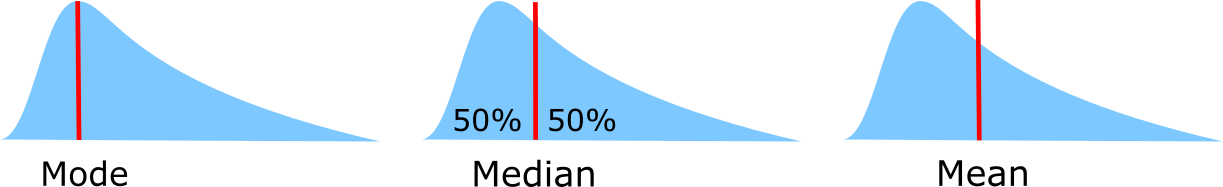
- Mode
- Most common value
- Median
- Central Value (less sensitive to outliers)
- Mean
- Sum observations / number of observations
Measuring Variability
- Range
- Largest observation – smallest observation
- Quantiles
- Split data like into equally numbered groups. Median into two, quartiles into 4
- Interquartile Range
- Range between top and bottom quartile. Shows where the middle 50% of the data lies. Not influenced by outliers
- Standard Deviation
Average deviation from the mean. Measures homogeneity of individual values.
\[std = \sqrt{\frac{\sum(x_i-x_{mean})^2}{n-1}}\]
Distribution
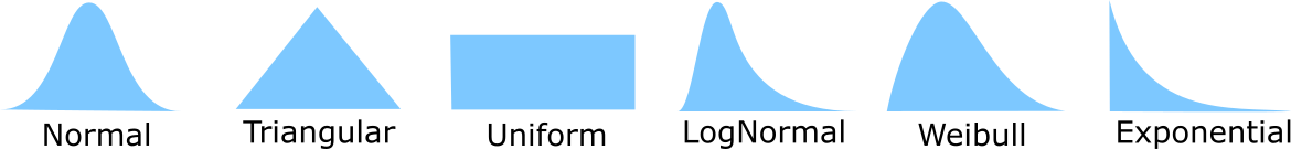
Some distributions
- Normal (=Gaussian) distribution
- Most common, unimodal, symmetrical. Other distributions tend to normalize when we increase sample size. Entirely defined by two parameters: means and std.
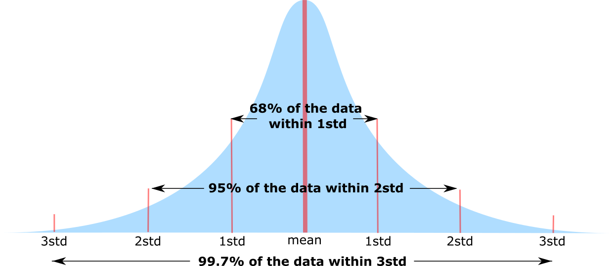
Normal Distribution
See the Statistical Tests section for info on testing or visualizing a distribution vs another.
- Law Of Large Numbers
- As a sample size grows, its mean will get closer and closer to the average of the whole population.
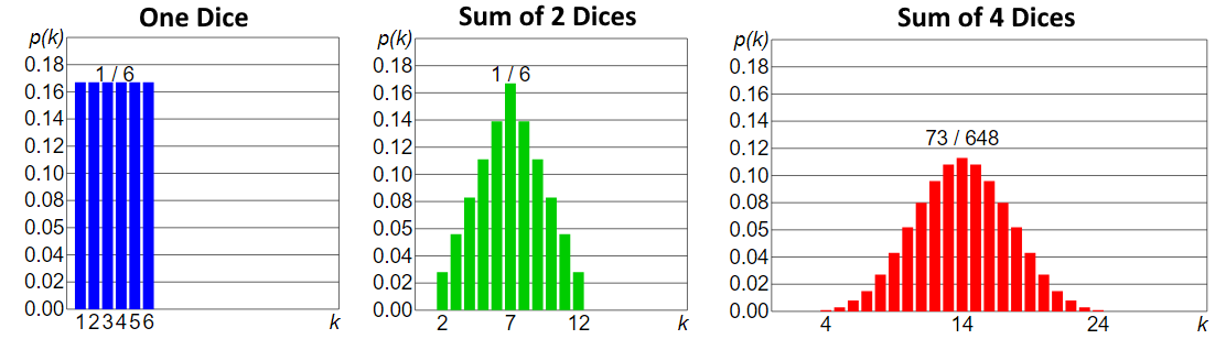
- Central Limit Theorem
- In probability theory, the central limit theorem (CLT) establishes that, in some situations, when independent random variables are added, their properly normalized sum tends toward a normal distribution even if the original variables themselves are not normally distributed. The theorem is a key concept in probability theory because it implies that probabilistic and statistical methods that work for normal distributions can be applicable to many problems involving other types of distributions.
Central Limit Theorem (wiki)
- Standard Error
Standard deviation of the sampling distribution of a statistic, most commonly of the mean. It can be seen as how far the sample mean is likely to be from the population mean
\[SE = \frac{std}{\sqrt{n}}\]- 95% Confidence Interval
For a gaussian distribution, the range in which 95% of the true population mean is likely to lie is defined by:
\[CI = [mean-1.96*\frac{std}{\sqrt{n}} , mean+1.96*\frac{std}{\sqrt{n}}]\]
1.96 can be replaced by other values for different percentages: 99%:2.576, 98%:2.326, 95%:1.96, 90%:1.645
May not be good for small sample size (<30) and very non normal distributions. In that case we can use the t-distribution to replace the 1.96
Correlation
See Statistical Tests to choose the appropriate method. TODO ADD MEAT TO CORRELATION
- Per Cohen (1992, Power primer):
- 0.0 < abs(corr) < 0.3: Weak 0.3 < abs(corr) <= 0.5: Moderate 0.5 < abs(corr) <= 0.9: Strong 0.9 < abs(corr) <= 1.0: Very strong
We can use a scatter plot to visualize correlation.